2.1.1. Manufacturer-Supplier Dynamical Network Simulation.

This function simulates a Manufacturer-Supplier (MS) dynamical network.

dynamical_networks.simulate.MS_network.MS_network(A_MS, M_arr, S_arr, make_gif=False, make_graph_plot=False)

This function takes system parameters to develop a time dependent adjacency matrix A(t).

Parameters

• A_MS (array) – Unweighted adjacency matrix for network.

• M_arr (array) – Throughput array for manufacturers.

• S_arr (array) – Throughput array for suppliers.

Kwargs:

plotting (bool): Plotting for user interpretation. defaut is False.

Returns

A, an n by n matrix A over time t.

Return type

(matrix)

dynamical_networks.simulate.MS_network.MS_simulation(t, parameters)

This function takes system parameters to develop a time dependent throughput simulation of manufacturers and suppliers.

Parameters

• parameter (float) – system parameter or parameters.

• t (array) – time array for simulation.

Kwargs:

plotting (bool): Plotting for user interpretation. defaut is False.

Returns

Arrays of t for the throughput of manufacturers and suppliers.

Return type

(M and S arrays)

The following is an example simulation of the supplier-manufacturer dynamical network:

from dynamical_networks.simulate.MS_network import MS_simulation, MS_network
import numpy as np
import matplotlib.pyplot as plt


#----------------------System Parameters and intial conditions------------------------
M = np.zeros((3,))+0.7                     #current throughput of manufacturer
S = np.zeros((2,))+0.8                      #current throughput of supplier
m = len(M)
s = len(S)
a = np.ones(s*m)
a[:int((m*s)*0.65)] = 0
np.random.shuffle(a)
A_MS = a.reshape((m,s))        #adjacency matrix for M/S connections
for i in range(len(A_MS)):
    if np.sum(A_MS[i]) == 0:
        j = int(np.random.uniform(0,len(A_MS[i]),1))
        A_MS[i][j] = 1
for i in range(len(A_MS.T)):
    if np.sum(A_MS.T[i]) == 0:
        j = int(np.random.uniform(0,len(A_MS.T[i]),1))
        A_MS[j][i] = 1

K_M = np.zeros((m,))+2      #maximum throughput of manufacturer
K_S = np.zeros((s,))+1       #maximum throughput of supplier
alpha_M = 0.01                     #internal perturbation of manufacturer
alpha_S = 0.01                      #internal perturbation of supplier
B_M1 = np.zeros((m,m))+0.6         #effects of price competition on manufacturer
B_S1 = np.zeros((s,s))+0.6        #effects of price competition on supplier
B_M2 = np.zeros((m,m))+0.0          #effects of technology competition on manufacturer
B_S2 = np.zeros((s,s))+0.0          #effects of technology competition on supplier
mu_M = np.zeros((m,))               #Manufacturer production outsourcing intensity
mu_S = np.zeros((s,))               #Supplier production outsourcing intensity
h = 2



# package parameters and define time array
parameters = [M, K_M, alpha_M, B_M1, B_M2, mu_M,S, K_S, alpha_S, B_S1, B_S2, mu_S, h, A_MS]
fs, L = 300, 15
t = np.linspace(0, L,int(L*fs))



#run simulation
M_arr, S_arr = MS_simulation(t, parameters)
A = MS_network(A_MS, M_arr, S_arr)



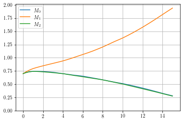
#plot resulting simulation throughput
for i in range(len(M_arr[0])):
    plt.plot(t, M_arr.T[i], label = r'$M_{'+str(i)+'}$')
plt.legend()
plt.ylim(0,)
plt.grid()
plt.show()

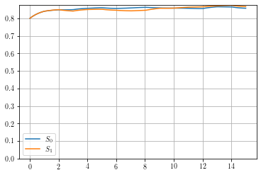
for i in range(len(S_arr[0])):
    plt.plot(t, S_arr.T[i], label = r'$S_{'+str(i)+'}$')
plt.legend()
plt.ylim(0,)
plt.grid()
plt.show()

Where the output for this example is:

Figure results for M_arr and S_arr